Quick Start

If you have not installed ITU-Rpy yet take a look at the installation instructions and make sure that all the requirements are fulfilled. Examples to illustrate the usage of ITU-Rpy are provided in the examples-folder. In order to understand the models used, check the models section .

To get started, we will walk you through a few examples that show the most illustrative case studies for

• First, we explain the basic usage of ITU-Rpy by computing the attenuation at a single location.
• Second, we explain the usage of ITU-Rpy using vectorized operations.
• Finally, we summarize other useful atmospheric functions in the library. The complete API description can be accessed through the API section .

Single location attenuation

Here we will compute the link attenuation vs. at a frequency of 22.5 GHz for a link between a satellite in GEO at the orbital slot 77 W and a ground station in Boston.

In addition, we will show how to compute other parameters of interest such as 0 degree isotherm, rainfall intensity exceeded during 0.01 % of the time, total columnar content liquid water or temperature.

First, let’s define the coordinates of our ground station and compute the elevation angle of the link

import itur
import astropy.units as u

# Ground station coordinates (Boston)
lat_GS = 42.3601
lon_GS = -71.0942

# Satellite coordinates (GEO, 77 W)
lat_sat = 0
lon_sat = -77
h_sat = 35786 * u.km

# Compute the elevation angle between satellite and ground station
el = itur.utils.elevation_angle(h_sat, lat_sat, lon_sat, lat_GS, lon_GS)

Next, we define the link parameters

f = 22.5 * u.GHz    # Link frequency
D = 1.2 * u.m       # Antenna diameters

Finally, we compute the total atmospheric attenuation as well as the different contributions for a set of unavailability values and plot the results. Note the flag return_contributions = True when calling function itur.atmospheric_attenuation_slant_path.

import numpy as np
import matplotlib.pyplot as plt
from matplotlib.ticker import ScalarFormatter

# Define unavailabilities vector
unavailabilities = np.logspace(-1.5, 1.5, 100)

# Compute the
A_g, A_c, A_r, A_s, A_t = [], [], [], [], []
for p in unavailabilities:
        a_g, a_c, a_r, a_s, a_t = itur.atmospheric_attenuation_slant_path(lat_GS, lon_GS,
                                                                          f, el, p, D,
                                                                          return_contributions=True)
        A_g.append(a_g.value)
        A_c.append(a_c.value)
        A_r.append(a_r.value)
        A_s.append(a_s.value)
        A_t.append(a_t.value)

# Plot the results
ax = plt.subplot(1,1,1)
ax.semilogx(unavailabilities, A_g, label='Gaseous attenuation')
ax.semilogx(unavailabilities, A_c, label='Cloud attenuation')
ax.semilogx(unavailabilities, A_r, label='Rain attenuation')
ax.semilogx(unavailabilities, A_s, label='Scintillation attenuation')
ax.semilogx(unavailabilities, A_t, label='Total atmospheric attenuation')

ax.xaxis.set_major_formatter(ScalarFormatter())
ax.set_xlabel('Percentage of time attenuation value is exceeded [%]')
ax.set_ylabel('Attenuation [dB]')
ax.grid(which='both', linestyle=':')
plt.legend()

which results in the following plot image:

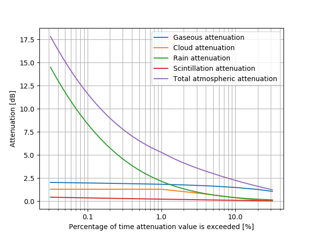
Atmospheric attenuation at Boston for a link to GEO - 77 W.

Note the by default, ITU-Rpy returns Quantity type objects, which are based on astropy.units module. Quantity objects are special objects that contain a value and unit attributes. Conversion among units is possible using the .to() method.

Atmospheric parameters such as temperature, pressure, or water-vapor density can be passed to function itur.atmospheric_attenuation_slant_path manually if known, otherwise ITU-Rpy will compute them automatically using the appropriate ITU Recommendation models. Similarly, if the ground station height above mean sea level is known, it can also be introduced manually.

Vectorial operations

One of the main characteristics of ITU-Rpy is that it allows for broadcasting of operations when using vectors. This allows for several use cases.

Multiple cities

First, we might be interested in computing the atmospheric attenuation values exceeded for 0.1 % of the time for a bunch of locations. This can be done as:

import itur
cities = {'Boston': (42.36, -71.06),
          'New York': (40.71, -74.01),
          'Los Angeles': (34.05, -118.24),
          'Denver': (39.74, -104.99),
          'Las Vegas': (36.20, -115.14),
          'Seattle': (47.61, -122.33),
          'Washington DC': (38.91, -77.04)}

lat = [coords[0] for coords in cities.values()]
lon = [coords[1] for coords in cities.values()]

# Satellite coordinates (GEO, 4 E)
lat_sat = 0
lon_sat = -77
h_sat = 35786 * itur.u.km

# Compute the elevation angle between satellite and ground stations
el = itur.utils.elevation_angle(h_sat, lat_sat, lon_sat, lat, lon)

# Set the link parameters
f = 22.5 * itur.u.GHz    # Link frequency
D = 1.2 * itur.u.m       # Antenna diameters
p = 0.1                  # Unavailability (Values exceeded 0.1% of time)

# Compute the atmospheric attenuation
Ag, Ac, Ar, As, Att = itur.atmospheric_attenuation_slant_path(
        lat, lon, f, el, p, D, return_contributions=True)

and we can plot the results

# Plot the results
city_idx = np.arange(len(cities))
width = 0.15

fig, ax = plt.subplots(1, 1)
ax.bar(city_idx, Att.value, 0.6, label='Total atmospheric Attenuation')

ax.bar(city_idx - 1.5 * width, Ar.value, width, label='Rain attenuation')
ax.bar(city_idx - 0.5 * width, Ag.value, width, label='Gaseous attenuation')
ax.bar(city_idx + 0.5 * width, Ac.value, width, label='Clouds attenuation')
ax.bar(city_idx + 1.5 * width, As.value, width,
           label='Scintillation attenuation')

# Set the labels
ticks = ax.set_xticklabels([''] + list(cities.keys()))
for t in ticks:
        t.set_rotation(45)
ax.set_ylabel('Atmospheric attenuation exceeded for 0.1% [dB]')

# Format image
ax.yaxis.grid(which='both', linestyle=':')
ax.legend(loc='upper center', bbox_to_anchor=(0.5, 1.3), ncol=2)
plt.tight_layout(rect=(0, 0, 1, 0.85))

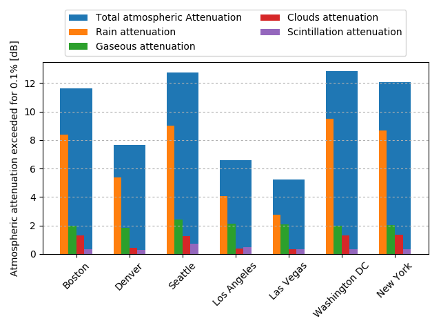
Atmospheric attenuation exceeded for 0.1 % of the average year in different cities of the US.

Attenuation over regions of the Earth

A second use case for vectorization is computation of the atmospheric attenuation (and other parameters) over large geographical regions. Let’s say that we want to compute the attenuation over Africa of a new Ka-band satellite located in GEO at slot 4 E.

import itur
import astropy.units as u

# Generate regular grid of latitude and longitudes with 1 degree resolution
lat, lon = itur.utils.regular_lat_lon_grid(lat_max=60,
                                           lat_min=-60,
                                           lon_max=65,
                                           lon_min=-35)

# Satellite coordinates (GEO, 4 E)
lat_sat = 0
lon_sat = 4
h_sat = 35786 * u.km

# Compute the elevation angle between satellite and ground station
el = itur.utils.elevation_angle(h_sat, lat_sat, lon_sat, lat, lon)

f = 22.5 * u.GHz    # Link frequency
D = 1.2 * u.m       # Antenna diameters
p = 1               # Unavailability (Values exceeded 1% of time)
Att = itur.atmospheric_attenuation_slant_path(lat, lon, f, el, p, D)

If you have installed Basemap (see installation instructions ), you can use function itur.plotting.plot_in_map() to display the results as an image:

# Plot the results
m = itur.plotting.plot_in_map(Att.value, lat, lon,
                           cbar_text='Atmospheric attenuation [dB]',
                           cmap='magma')

# Plot the satellite location
m.scatter(lon_sat, lat_sat, c='white', s=20)

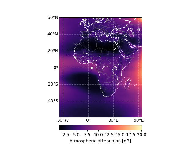
Atmospheric attenuation over Africa @ 22.5 GHz.

Dependency with link parameters

Vectorization works in a lot of different ways. For example, let’s say that we want to compute the dependency of the attenuation with the elevation angle for a the example presented in the `Single location attenuation example <>`_. We can just do it using the code below

import itur
import astropy.units as u

itur.deactivate_output_quantity()

# Ground station coordinates (Boston)
lat_GS = 42.3601
lon_GS = -71.0942

# Vectorize the elevation angle
el = np.linspace(10, 90, 50)

f = 22.5 * u.GHz    # Link frequency
D = 1.2 * u.m       # Antenna diameters
p = 1               # Unavailability (Values exceeded 1% of time)
Att = itur.atmospheric_attenuation_slant_path(lat_GS, lon_GS, f, el, p, D)

plt.figure()
plt.plot(el, Att.value)
plt.xlabel('Elevation angle [deg]')
plt.ylabel('Attenuation [dB]')
plt.grid(which='major', linestyle=':')

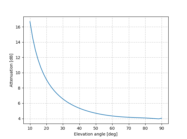
Atmospheric attenuation at Boston vs. elevation angle.

Another example of vectorization can be found below in the code to plot the atmospheric attenuation due to gases vs. frequency.

import itur
import astropy.units as u
import numpy as np

el = 90
rho = 7.5 * u.g / u.m**3
P = 1013 * u.hPa
T = 25 * u.deg_C
f = np.linspace(1, 350, 1000)

Att = itur.gaseous_attenuation_slant_path(f, el, rho, P, T)
plt.semilogy(f, Att)
plt.xlabel('Frequency [GHz]')
plt.ylabel('Gaseous Attenuation [dB]')
plt.grid(which='both', linestyle=':')

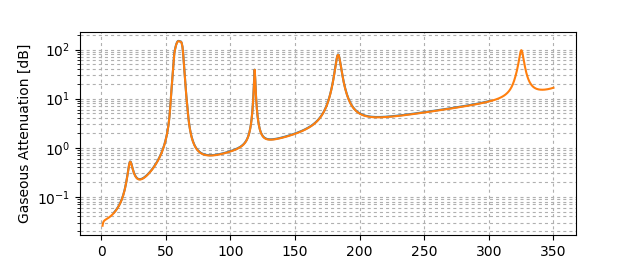
Gaseous attenuation vs. frequency.

The only parameter that cannot be vectorized is the unavailability - percentage of time that values are exceeded. A for loop needs always to be used to compute attenuation values for different unavailabilities (p), as was shown in the `Single location attenuation example <>`_.

Other atmospheric functions

We conclude the quickstart with a summary of other functions included in ITU-Rpy that might be useful to compute atmospheric attenuation related parameters. The complete API description can be accessed through the API section .

import itur

# Location of the receiver ground stations
lat = 41.39
lon = -71.05

# Link parameters
el = 60                # Elevation angle equal to 60 degrees
f = 22.5 * itur.u.GHz  # Frequency equal to 22.5 GHz
D = 1 * itur.u.m       # Receiver antenna diameter of 1 m
p = 0.1                # We compute values exceeded during 0.1 % of the average
                                           # year

# Compute atmospheric parameters
hs = itur.topographic_altitude(lat, lon)
T = itur.surface_mean_temperature(lat, lon)
P = itur.standard_pressure(lat, hs)
rho_p = itur.surface_water_vapour_density(lat, lon, p, hs)
rho_sa = itur.models.itu835.water_vapour_density(lat, hs)
T_sa = itur.models.itu835.temperature(lat, hs)
V = itur.models.itu836.total_water_vapour_content(lat, lon, p, hs)

# Compute rain and cloud-related parameters
R_prob = itur.models.itu618.rain_attenuation_probability(lat, lon, el, hs)
R_pct_prob = itur.models.itu837.rainfall_probability(lat, lon)
R001 = itur.models.itu837.rainfall_rate(lat, lon, p)
h_0 = itur.models.itu839.isoterm_0(lat, lon)
h_rain = itur.models.itu839.rain_height(lat, lon)
L_red = itur.models.itu840.columnar_content_reduced_liquid(lat, lon, p)
A_w = itur.models.itu676.zenit_water_vapour_attenuation(lat, lon, p, f, alt=hs)

# Compute attenuation values
A_g = itur.gaseous_attenuation_slant_path(f, el, rho_p, P, T)
A_r = itur.rain_attenuation(lat, lon, f, el, hs=hs, p=p)
A_c = itur.cloud_attenuation(lat, lon, el, f, p)
A_s = itur.scintillation_attenuation(lat, lon, f, el, p, D)
A_t = itur.atmospheric_attenuation_slant_path(lat, lon, f, el, p, D)

Running the code above produces the following results. The ITU Recommendation where the variable or the procedure to compute it is referred appears in square brackets.

The ITU recommendations predict the following values for the point located
at coordinates (41.39, -71.05)
  - Height above the sea level                  [ITU-R P.1511]      22.9 m
  - Surface mean temperature                    [ITU-R P.1510]      9.4 deg_C
  - Surface pressure                            [ITU-R P.835]       1005.4 hPa
  - Standard surface temperature                [ITU-R P.835]       13.6 deg_C
  - Standard water vapour density               [ITU-R P.835]       8.9 g / m3
  - Water vapor density (p=0.1%)                [ITU-R P.836]       20.3 g / m3
  - Total water vapour content (p=0.1%)         [ITU-R P.836]       54.6 kg / m2
  - Rain attenuation probability                [ITU-R P.618]       9.6 %
  - Rain percentage probability                 [ITU-R P.837]       7.8 %
  - Rainfall rate exceeded for p=0.1%           [ITU-R P.837]       12.9 mm / h
  - 0 degree C isotherm height                  [ITU-R P.839]       3.2 km
  - Rain height                                 [ITU-R P.839]       3.5 km
  - Columnar content of reduced liquid (p=0.1%) [ITU-R P.840]       3.0 kg / m2
  - Zenit water vapour attenuation (p=0.1%)     [ITU-R P.676]       1.5 dB


Attenuation values exceeded for p=0.1% of the average year for a link with el=60 deg, f=22.5 GHz,
D=1.0 m and receiver ground station located at coordinates (41.39, -71.05)
  - Rain attenuation                            [ITU-R P.618]       8.2 dB
  - Gaseous attenuation                         [ITU-R P.676]       1.5 dB
  - Clouds attenuation                          [ITU-R P.840]       1.6 dB
  - Scintillation attenuation                   [ITU-R P.618]       0.3 dB
  - Total atmospheric attenuation               [ITU-R P.618]       10.8 dB